42 row labels in excel pivot table
How to make row labels on same line in pivot table? - ExtendOffice Click any cell in your pivot table, and the PivotTable Tools tab will be displayed. 2. Under the PivotTable Tools tab, click Design > Report Layout > Show in Tabular Form, see screenshot: 3. And now, the row labels in the pivot table have been placed side by side at once, see screenshot: Group PivotTable Data by Sepcial Time Multiple row labels on one row in Pivot table - MrExcel Message Board In Excel 2003, a pivot table would allow you to place multiple row labels on the left hand side of a pivot table. I can't figure out how to make that happen in Excel 2010. I need material and material description on the lefthand side of the pivot table but it is placing the description underneath on a 2nd row form the material number.
Excel: How to Filter Data in Pivot Table Using “Greater Than” May 05, 2022 · Often you may want to filter values in a pivot table in Excel using a “Greater Than” filter. Fortunately this is easy to do using the Value Filters dropdown menu within the Row Labels column of a pivot table. The following example shows exactly how to do so. Example: Filter Data in Pivot Table Using “Greater Than”

Row labels in excel pivot table
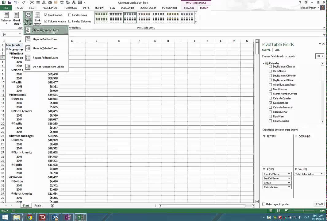
Data Labels in Excel Pivot Chart (Detailed Analysis) 7 Suitable Examples with Data Labels in Excel Pivot Chart Considering All Factors 1. Adding Data Labels in Pivot Chart 2. Set Cell Values as Data Labels 3. Showing Percentages as Data Labels 4. Changing Appearance of Pivot Chart Labels 5. Changing Background of Data Labels 6. Dynamic Pivot Chart Data Labels with Slicers 7. Design the layout and format of a PivotTable To change the layout of a PivotTable, you can change the PivotTable form and the way that fields, columns, rows, subtotals, empty cells and lines are displayed. To change the format of the PivotTable, you can apply a predefined style, banded rows, and conditional formatting. Windows Web Mac Changing the layout form of a PivotTable Pivot table row labels in separate columns • AuditExcel.co.za Our preference is rather that the pivot tables are shown in tabular form (all columns separated and next to each other). You can do this by changing the report format. So when you click in the Pivot Table and click on the DESIGN tab one of the options is the Report Layout. Click on this and change it to Tabular form.
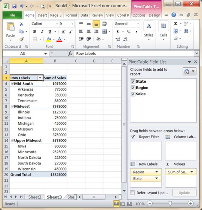
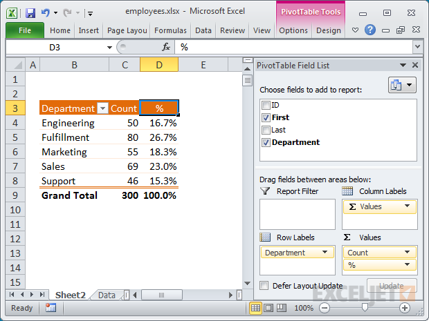
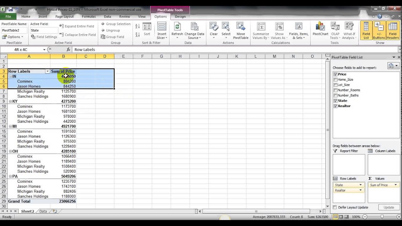
Row labels in excel pivot table. Pivot Table Row Labels - Microsoft Community If you go to PivotTable Tools > Analyze > Layout > Report Layout > Show in Tabular Form, your column headers will be used for the row labels. Every once in a while there's a sudden gust of gravity... Report abuse 1 person found this reply helpful · Was this reply helpful? Yes No A. User Replied on December 19, 2017 excel - Custom row labels in PivotTable - Stack Overflow 1 you can give nicknames to the fields that you are checking which populate the pivot table. If you go the pivot table data and right click you can change the value field settings to give a custom name to a row/series but I do not know about individual data points. path: pivot table data => right click => select Field Settings => edit custom name. Automatic Row And Column Pivot Table Labels - How To Excel At Excel The first thing to do is put your cursor somewhere in your data list Select the Insert Tab Hit Pivot Table icon Next select Pivot Table option Select a table or range option Select to put your Table on a New Worksheet or on the current one, for this tutorial select the first option Click Ok Move Row Labels in Pivot Table - Excel Pivot Tables When you add fields to the row labels area in a pivot table, the field's items are automatically sorted. See how you can manually move those labels, to put them in a different order. There's a video and written steps below. In the screen shot below, the districts are listed alphabetically, from Central to West. Change the Order
Pivot Table "Row Labels" Header Frustration Pivot Table "Row Labels" Header Frustration. Hi Everyone please help I can't change my headers from Row Labels in a Pivot Table. Using Excel 365. Labels: Row labels not showing correctly in pivot table Re: Row labels not showing correctly in pivot table. You can't rename a row or column header to a name that is part of the data, but you can easily type in the same name with a leading or trailing space. One spreadsheet to rule them all. One spreadsheet to find them. One spreadsheet to bring them all and at corporate, bind them. Sorting to your Pivot table row labels in custom order [quick tip] Add sort order column along with classification to the pivot table row labels area. Add the usual stuff to values area. Set up pivot table in tabular layout. Remove sub totals; Finally hide the column containing sort order. Your new pivot report is ready. Good news for people with Excel 2013 or above: How to make row labels on same line in pivot table? - ExtendOffice In Excel, when you create a pivot table, the row labels are displayed as a compact layout, all the headings are listed in one column. Sometimes, you need to convert the compact layout to outline form to make the table more clearly. This article will tell you how to repeat row labels for group in Excel PivotTable.
MS Excel 2016: How to Create a Pivot Table - TechOnTheNet Steps to Create a Pivot Table. To create a pivot table in Excel 2016, you will need to do the following steps: Before we get started, we first want to show you the data for the pivot table. In this example, the data is found on Sheet1. Highlight the cell where you'd like to create the pivot table. In this example, we've selected cell A1 on Sheet2. Sort pivot table values with multiple row labels Re: Sort multiple row label in pivot table. Originally Posted by MarvinP. Yes, I do believe you can sort by values. Using Excel 2010 click on the Opportunity ID drop down and select "More Sort Options" From there choose the dropdown and "Sum of Values". See attached. Select the Insert Tab. Hit Pivot Table icon. Next select Pivot Table option. How to repeat row labels for group in pivot table? - ExtendOffice Firstly, you need to expand the row labels as outline form as above steps shows, and click one row label which you want to repeat in your pivot table. 2. Then right click and choose Field Settings from the context menu, see screenshot: 3. In the Field Settings dialog box, click Layout & Print tab, then check Repeat item labels, see screenshot: 4. How to rename group or row labels in Excel PivotTable? - ExtendOffice To rename Row Labels, you need to go to the Active Field textbox. 1. Click at the PivotTable, then click Analyze tab and go to the Active Field textbox. 2. Now in the Active Field textbox, the active field name is displayed, you can change it in the textbox. You can change other Row Labels name by clicking the relative fields in the PivotTable ...
Pivot Table Row Labels In the Same Line - Beat Excel!
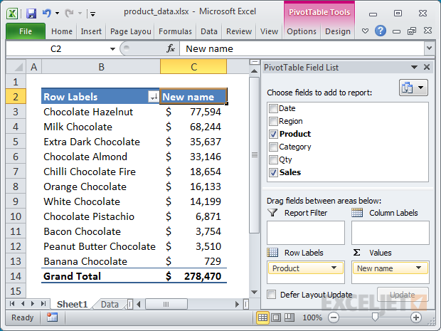
Change the pivot table "Row Labels" text | MrExcel Message Board 144. Feb 4, 2021. #3. mart37 said: Click on the cell and typ the text. Thanks mart37. So simple! I was looking for a way to change it on the ribbons & settings. Typical Excel - things you think are difficult are easy, and things that should be easy are difficult!

Microsoft Excel – showing field names as headings rather than ...
How to Format Excel Pivot Table - Contextures Excel Tips Jun 22, 2022 · Video: Change Pivot Table Labels. Watch this short video tutorial to see how to make these changes to the pivot table headings and labels. Get the Sample File. No Macros: To experiment with pivot table styles and formatting, download the sample file. The zipped file is in xlsx format, and and does NOT contain any macros.

Pivot table row labels side by side – Excel Tutorials
get a row label from pivot table - Microsoft Tech Community Creating PivotTable add data to data model by checking Create PivotTable and after that convert it to cube formulas. Now you may take these formulas and convert it to form you need, for example in H3 it could be =CUBEVALUE( "ThisWorkbookDataModel", CUBEMEMBER("ThisWorkbookDataModel", " [Measures].
Help Online - Origin Help - Pivot Table
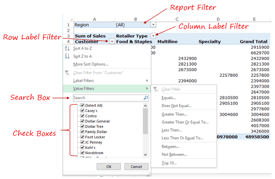
How to Use Excel Pivot Table Date Range Filter- Steps, Video Jun 22, 2022 · Pivot Table in Compact Layout. If your pivot table is in Compact Layout, all of the Row fields are in a single column. The column heading says "Row Labels". To choose the pivot field that you want to filter, follow these steps: In the pivot table, click the drop down arrow on the Row Labels heading; In the Select Field box, slick the drop down ...

Permanently Tabulate Pivot Table Report & Repeat All Item ...
How to Group Numbers in Pivot Table in Excel - Trump Excel Sometimes, numbers are stored as text in Excel. In such case, you need to convert these text to numbers before grouping it in Pivot Table. You May Also Like the Following Pivot Table Tutorials: How to Group Dates in Pivot Table in Excel. How to Create a Pivot Table in Excel. Preparing Source Data For Pivot Table. How to Refresh Pivot Table in ...

Changing Order of Row Labels in Pivot Table
Pivot table row labels side by side - Excel Tutorials - OfficeTuts Excel You can copy the following table and paste it into your worksheet as Match Destination Formatting. Now, let's create a pivot table ( Insert >> Tables >> Pivot Table) and check all the values in Pivot Table Fields. Fields should look like this. Right-click inside a pivot table and choose PivotTable Options…. Check data as shown on the image below.

Pivot Table column label from horizontal to vertical ...
Automate Pivot Table with Python (Create, Filter and Extract) 22.05.2021 · Photo by Jasmine Huang on Unsplash. In Automate Excel with Python, the concepts of the Excel Object Model which contain Objects, Properties, Methods and Events are shared.The tricks to access the Objects, Properties, and Methods in Excel with Python pywin32 library are also explained with examples.. Now, let us leverage the automation of Excel report …

In pivot tables how can I replace Row Labels with field names ...
How to Use Excel Pivot Table Label Filters - Contextures Excel Tips To do that, you could click the drop down arrow for the Row or Column Labels, to see the list of pivot items in that pivot field. Then, in the list, remove the check mark for items you want to remove. For example, to hide the data for 7-Feb-10, you'd click on the check mark to remove it.
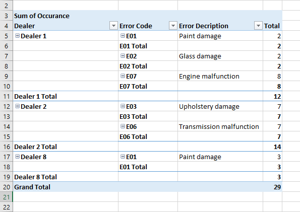
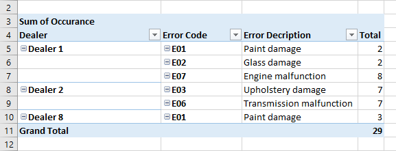
How to Flatten and repeat Row Labels in a Pivot Table
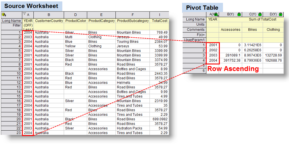
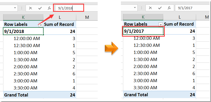
Excel Pivot Table Report Filter Tips and Tricks - Contextures Excel … Jul 14, 2022 · To enable the grouping command, you’ll temporarily move the Report Filter field to the Row Labels area. In the screen shot below, the OrderDate field is being dragged to the Row Labels area, in the PivotTable fields pane. Then, right-click on the field in the pivot table, and click Group. Select the Grouping options that you want, and click OK

Remove filter from ROW LABELS on pivot table Excel - Super User
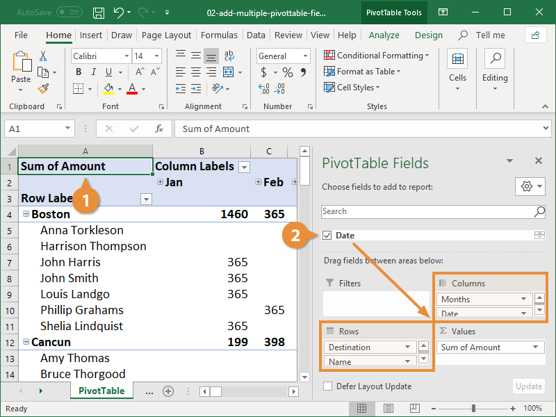
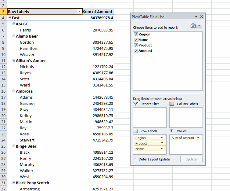
multiple fields as row labels on the same level in pivot table Excel ... multiple fields as row labels on the same level in pivot table Excel 2016. I am using Excel 2016. I have data that lists product models along with relevant data and also production volumes by month. Part of the relevant data are about 5 common part columns with the part # that applies to each model under the appropriate column.

Excel Tips: Repeat Row Labels in Excel 2007
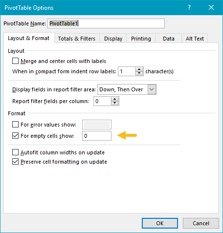
How to insert a blank column in pivot table? - Chandoo.org 16.04.2015 · We all know pivot table functionality is a powerful & useful feature. But it comes with some quirks. For example, we cant insert a blank row or column inside pivot tables. So today let me share a few ideas on how you can insert a blank column. But first let's try inserting a column Imagine you are looking at a pivot table like above. And you want to insert a column or row. …
Excel PivotTable Percentage: Which Customers Are Costing You ...
Multi-row and Multi-column Pivot Table - Excel Start Once the pivot table sheet is created, just like in the previous example, drag the Category and the Product to the Rows section and the Sales Value to the Values section to get the same Multi-Row pivot table we did in the previous example. Next we want to add a column. We will add the Date to the Column section by dragging the field.
Design the layout and format of a PivotTable
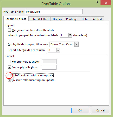
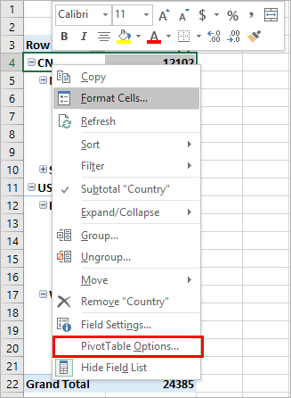
Remove row labels from pivot table • AuditExcel.co.za Click on the Pivot table. Click on the Design tab. Click on the report layout button. Choose either the Outline Format or the Tabular format. If you like the Compact Form but want to remove 'row labels' from the Pivot Table you can also achieve it by. Clicking on the Pivot Table. Clicking on the Analyse tab.
Microsoft Excel Training in Columbus | Make Tech Easy With EasyIT
Quick tip: Rename headers in pivot table so they are presentable Mar 15, 2018 · If you love working with pivot tables, check out below tips to become even more awesome. Sub-totals for only some levels; Change the order of pivot table row labels; First and last date of a sale with pivots; Introduction to pivot tables; Pivots from multiple tables; What is your favorite pivot tip? Please share in comments.

Excel pivot table shows only when rows have multiple other ...
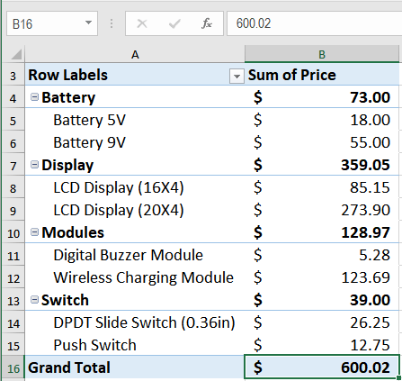
How to Group Rows in Excel Pivot Table (3 Ways) - ExcelDemy Now select any number in the Row Labels of the table. Then right-click and select Group as shown below. Then, enter the Starting ( 60) and Ending ( 100) numbers and the difference ( 10) by which you want to group them. Next, hit OK. Finally, you will see the numbers grouped together as shown in the picture below.👇.
Pivot table row labels side by side – Excel Tutorials
How to Group Data in Pivot Table (3 Simple Methods) Step 01: Insert a Pivot Table Firstly, select the dataset as shown below and click on the Insert ribbon. Then, you'll find the PivotTable drop-down on the right where you need to select the From Table/Range option. Next, a dialog box appears in which you have to check the New Worksheet option and press OK. Step 02: Construct Pivot Table

Identifying the Pivot Table fields for each row (Excel ...
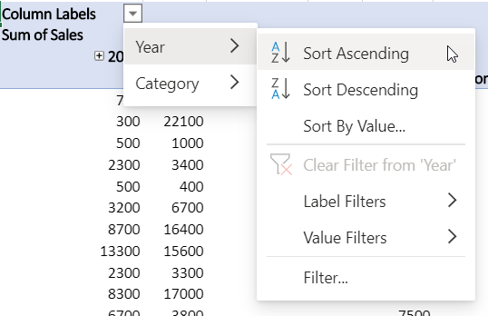
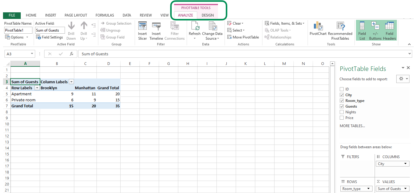
Excel tutorial: How to filter a pivot table by rows or columns When you add a field as a row or column label in a pivot table, you automatically get the ability to filter the results in the table by items that appear in that field. Let's take a look. This pivot table is displaying just one field: Total Sales. After we add Product as a row label, notice that a drop-down arrow appears in the header area.

Ranking in excel pivot table with 2 dimensions/row labels : r ...
How to rename group or row labels in Excel PivotTable? - ExtendOffice To rename Row Labels, you need to go to the Active Field textbox. 1. Click at the PivotTable, then click Analyze tab and go to the Active Field textbox. 2. Now in the Active Field textbox, the active field name is displayed, you can change it in the textbox.

Repeat Pivot Table row labels • AuditExcel.co.za Pivot Tables ...
How to group time by hour in an Excel pivot table? - ExtendOffice Now the pivot table is added. Right-click any time in the Row Labels column, and select Group in the context menu. See screenshot: 5. In the Grouping dialog box, please click to highlight Hours only in the By list box, and click the OK button. See screenshot: Now the time data is grouped by hours in the newly created pivot table. See screenshot:
Pivot Table Tips | Exceljet
Repeat item labels in a PivotTable - support.microsoft.com Right-click the row or column label you want to repeat, and click Field Settings. Click the Layout & Print tab, and check the Repeat item labels box. Make sure Show item labels in tabular form is selected. Notes: When you edit any of the repeated labels, the changes you make are applied to all other cells with the same label.

Pivot table row labels side by side – Excel Tutorials
Pivot table row labels in separate columns • AuditExcel.co.za Our preference is rather that the pivot tables are shown in tabular form (all columns separated and next to each other). You can do this by changing the report format. So when you click in the Pivot Table and click on the DESIGN tab one of the options is the Report Layout. Click on this and change it to Tabular form.

EXCEL: SETTING PIVOT TABLE DEFAULTS - Strategic Finance
Design the layout and format of a PivotTable To change the layout of a PivotTable, you can change the PivotTable form and the way that fields, columns, rows, subtotals, empty cells and lines are displayed. To change the format of the PivotTable, you can apply a predefined style, banded rows, and conditional formatting. Windows Web Mac Changing the layout form of a PivotTable
Pivot table row labels side by side – Excel Tutorials
Data Labels in Excel Pivot Chart (Detailed Analysis) 7 Suitable Examples with Data Labels in Excel Pivot Chart Considering All Factors 1. Adding Data Labels in Pivot Chart 2. Set Cell Values as Data Labels 3. Showing Percentages as Data Labels 4. Changing Appearance of Pivot Chart Labels 5. Changing Background of Data Labels 6. Dynamic Pivot Chart Data Labels with Slicers 7.
Add Multiple Columns to a Pivot Table | CustomGuide
The Pivot table tools ribbon in Excel

Adding a Calculated Item to a Pivot Table in Excel 2010
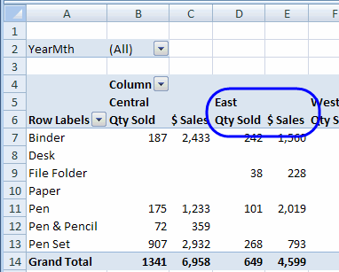
Pivot Table: Pivot table display items with no data | Exceljet
Centre Column Headings in Excel Pivot Table | Excel Pivot Tables
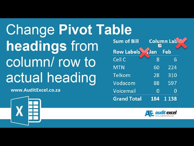
Pivot Table headings that say column/ row instead of actual ...
Multiple Row Filters in Pivot Tables
Pivot Table Tips | Exceljet
How to Use a Pivot Table in Excel

Pivot table row labels in separate columns • AuditExcel.co.za
My Biggest Pivot Table Annoyance (And How To Fix It ...

pivot table row labels in separate columns 2 • AuditExcel.co.za

How to make row labels on same line in pivot table?
How to Filter Data in a Pivot Table in Excel
How to rename group or row labels in Excel PivotTable?
Instructions for Transposing Pivot Table Data | Excelchat
How to make row labels on same line in pivot table?
Repeating Values in Pivot Tables – Daily Dose of Excel

Pivot table row labels in separate columns • AuditExcel.co.za
Post a Comment for "42 row labels in excel pivot table"